Categories
GoLang Web Application

Getting started with a Golang web application

Started looking at Golang about a year ago, reading through a few tutorials and writing some script sized programs. At the time I thought I would use Golang for specific sysadmin type tasks. It didn’t really pan out as the time to completion vs bash or python is almost always much lower. Scripting in bash and pythons means you can always fix bugs with just a text editor with no compiling – dependency management is pretty simple, on all linux distros. So I didn’t write anything in Golang for almost a year and forgot most of it! I have an idea for a business tool enabling mapping and execution of organisational objectives, strategy and operations.

Learning with a Project

The only way to learn a programming language is to use it on a project (or many). So I am building a web application that requires:

  • Authentication/Identification/Roles
  • Forms for input
  • Navigation/Searching/SIngle page
  • Charting/Models
  • Persistent data
  • Security controls such as csrf tokens

IDE

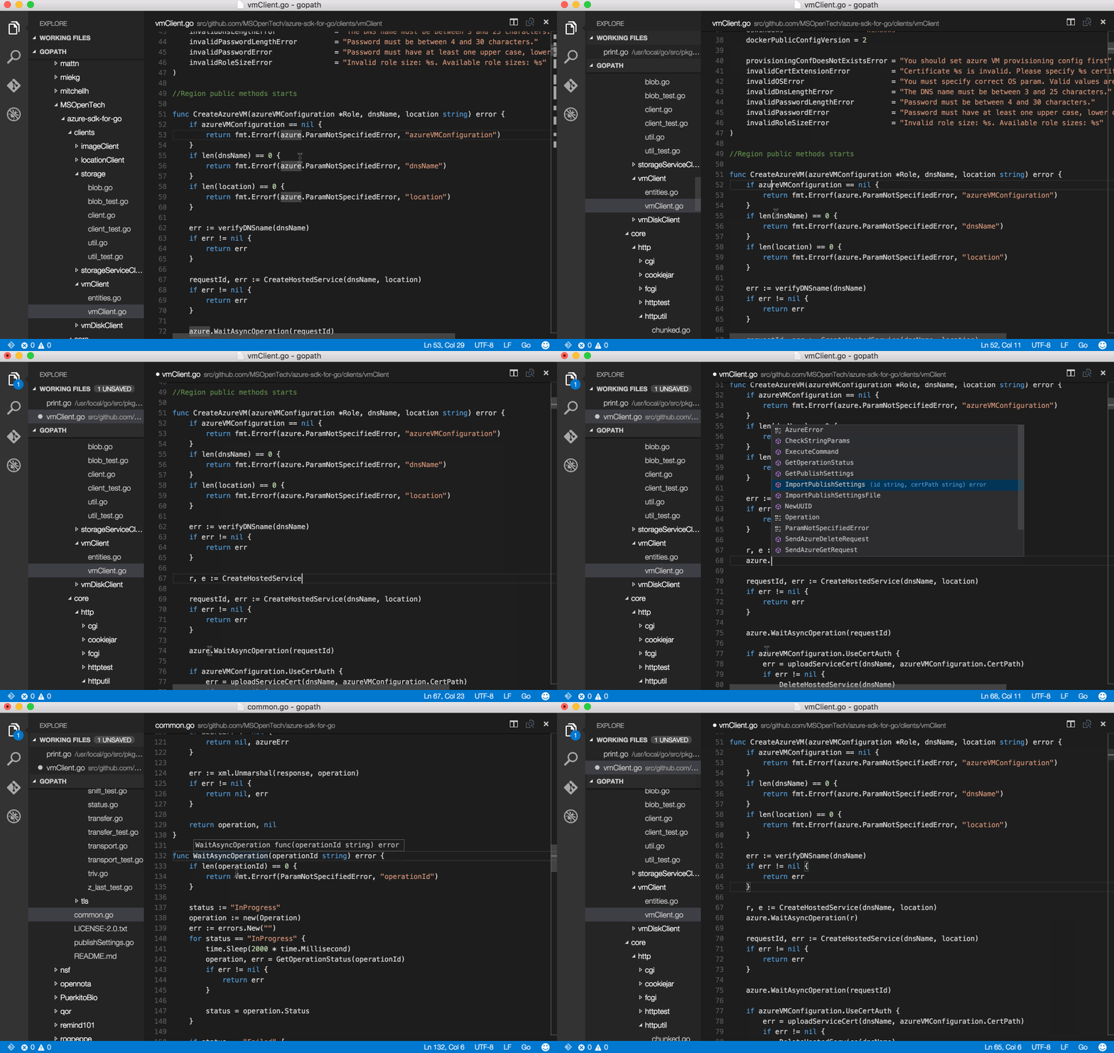
Previously I added a bunch of plugins to vim and managed a custom and complex vimrc file. I found that having to manage all of that on numerous workstations was too time expensive. So – in an effort for workstation portability and ease of management, I am trying the GoLand ide by JetBrains. I will decide after my 30 day trial whether or not to pay the 200 usd per year price tag. If it means I write code more often (not avoiding the environment setup, maintenance and portability issues) it may well be worth it. Ended up going with Microsoft Visual Code which is on linux, macos and windows, is opensource, free and quick and easy to set up.

After thinking about what I just wrote above – it is nonsense. I should just take 30 minutes to write down how to set up a decent Golang environment. Started but abandoned: https://mwclearning.com/?p=1858

Tutorial

https://golang.org/doc/articles/wiki/ is a nice short tutorial from the makers or Golang that introduces the basic concepts. That along with A tour of Go are enough to get started.

TechStack

Starting with:

  • Relational database backend (postgres)
  • Javascript frontend (vuejs)
  • Application code (Golang)
  • Framework (gin / echo)
  • Requirement tracking / Agile board (taskworld)
  • Source code management (gitlab.com – free private repos)
  • Integrate Development Environment (Microsoft Visual Code)

Getting started

Tutorials based on what I features are needed to meet requirements.
Categories
GoLang Web Application Random

Free Golang IDE (s) on macos (Visual Studio Code / vim)

Visual Studio Code

Visual Studio Code is a now is Microsoft’s now OpenSource IDE that runs on windows, macos and linux!

Simple set up guide here: https://rominirani.com/setup-go-development-environment-with-visual-studio-code-7ea5d643a51a. Assuming go is installed and ready to do – the download, install and setup took about 5 minutes. Everything just works out of the box and its much less dependency on complex config files and plugins (vs vim).


Vim (abandoned this for Microsoft Visual Code)

Install these if they are not already:

brew install vim
# Note that is is executing arbitrary code from an the vim-go repo 
curl -fLo ~/.vim/autoload/plug.vim --create-dirs https://raw.githubusercontent.com/junegunn/vim-plug/master/plug.vim 
git clone https://github.com/fatih/vim-go.git ~/.vim/plugged/vim-go
  • Customise ~/.vimrc to enable and configure your plugins and shortcut keys
  • Once th ~/.vimrc is added run :GoInstallBinaries to get vim-go’s dependencies

Shortcut keys in this vimrc:

  • \ + b -> build
    • if errors occur toggle forward and back through them with ctrl + n and ctrl + m
    • close quick fix dialogue boxes with \ + a
  • \ + i -> install
  • dif (whilst on func def, delete all contents for func)

Autocompletion sucks though 🙁 so adding neocomplete is a must).

With existing versions of brew installed vim and the introduced dependency of xcode makes the setup time high. I went through this in the past and after a fairly long hiatus from writing code if find nothing is working quite right.


Categories
Data Mining Project

Week 3 – Introduction to R. Cont’

Coming back to R after closing, a session can be restored by simply running R in the workspace directory.

A history file can be specified via:

# recall your command history 
loadhistory(file="myfile") # default is ".Rhistory"

RData can also be saved and loaded via:

# save the workspace to the file .RData in the cwd 
save.image()

# save specific objects to a file
# if you don't specify the path, the cwd is assumed 
save(object list,file="myfile.RData")
# load a workspace into the current session
# if you don't specify the path, the cwd is assumed 
load("myfile.RData")

Describing data:

# show data files attached
ls()
# show dimensions of  a data object 'd'
dim(d)
#show structure of data object 'd'
str(d)
#summary of data 'd'
summary(d)

Subsets of data is a logical next step:

summary(subset(d, read <= 60))

Grouping data is also fairly intuitive:

by(d[, 7:11], d$prog, colMeans)
by(d[, 7:11], d$prog, summary)

Using histograms to plot variable distributions:

ggplot(d, aes(x = write)) + geom_histogram()
# Or kernel density plots
ggplot(d, aes(x = write)) + geom_density()
# Or boxplots showing the median, lower and upper quartiles and the full range
ggplot(d, aes(x = 1, y = math)) + geom_boxplot()

Lets look at some more ways to understand the data set:

# density plots by program type
ggplot(d, aes(x = write)) + geom_density() + facet_wrap(~prog)
# box plot of math scores for each teaching program
ggplot(d, aes(x = factor(prog), y = math)) + geom_boxplot()

Extending visualizations:

ggplot(melt(d[, 7:11]), aes(x = variable, y = value)) + geom_boxplot()
# break down by program:
ggplot(melt(d[, 6:11], id.vars = "prog"), aes(x = variable, y = value, fill = factor(prog))) +  geom_boxplot()

Analysis of categories can be conducted with frequency tables:

xtabs(~female, data = d)
xtabs(~race, data = d)
xtabs(~prog, data = d)
xtabs(~ses + schtyp, data = d)

Finally lets have a look at some bivatiate (pairwise) correlations. If ther is no missing data, cor function can be users, else use can remove items:

cor(d[, 7:11])
ggpairs(d[, 7:11])


Categories
Data Mining Project

Week 2 – Introduction to R.

Why use R?

R is an integrated suite of software facilities for data manipulation, calculation and graphical display. – http://cran.csiro.au/doc/manuals/r-release/R-intro.html

This is a valid question considering that most languages/frameworks, including CUDA have statistical analysis libraries built in. Hopefully running through some introductory exercises will reveal the benefits.

Associated GUI’s and extensions:

  • Weka – Specific for machine learning algorithms
  • R Commander – Data analysis GUI

Install on Ubuntu 12.04:

  1. sudo echo "deb http://cran.csiro.au/bin/linux/ubuntu precise/" >> /etc/apt/sources.list
    sudo apt-get update
    sudo apt-get install r-base

    Then to enter the R command line interface, $ R

    For starters, will run through an intro from UCLA: http://www.ats.ucla.edu/stat/r/seminars/intro.htm

    Within the R command line interface if a package is to be used it must first be installed:

    install.packages()
    • foreign – package to read data files from other stats packages
    • xlsx – package (requires Java to be installed, same architecture as your R version, also the rJava package and xlsxjars package)
    • reshape2 – package to easily melt data to long form
    • ggplot2 – package for elegant data visualization using the Grammar of Graphics
    • GGally – package for scatter plot matrices
    • vcd – package for visualizing and analyzing categorical data
    install.packages("xlsx")
    install.packages("reshape2")
    install.packages("ggplot2")
    install.packages("GGally")
    install.packages("vcd")

    Pre-requisites:

    sudo apt-get install openjdk-7-*
    sudo ln -s /usr/lib/jvm/java-7-openjdk-amd64/bin/java /etc/alternatives/java
    sudo R CMD javareconf

    Preparing session:

    After installing R and the packages needed for a task if these packages are needed in the current session they must be included:

    require(foreign)
    require(xlsx)

    After attaching all of the required packages to the current session, confirmation can be completed via:

    sessionInfo()

    R code can be entered into the command line directly or saved to a script which can be run inside a session using the ‘source’ function.

    Help can be attained using ? preceding a function name.

    Entering Data:

    R is most compatible with datasets stored as text files, ie: csv.

    Base R contains functions read.table and read.csv see the help files on these functions for many options.

    # comma separated values
    dat.csv <- read.csv("http://www.ats.ucla.edu/stat/data/hsb2.csv")
    # tab separated values
    dat.tab <- read.table("http://www.ats.ucla.edu/stat/data/hsb2.txt", header=TRUE, sep = "\t")
    

    Datasets from other statistical analysis software can be imported using the foreign package:

    require(foreign)
    # SPSS files
    dat.spss <- read.spss("http://www.ats.ucla.edu/stat/data/hsb2.sav", to.data.frame=TRUE)
    # Stata files
    dat.dta <- read.dta("http://www.ats.ucla.edu/stat/data/hsb2.dta")

    If converting excel spreadsheets to CSV is too much of a hassle the xlxs package we imported will do the job:

    # these two steps only needed to read excel files from the internet
    f <- tempfile("hsb2", fileext=".xls")
    download.file("http://www.ats.ucla.edu/stat/data/hsb2.xls", f, mode="wb")
    dat.xls <- read.xlsx(f, sheetIndex=1)

    Viewing Data:

    # first few rows
    head(dat.csv)
    # last few rows
    tail(dat.csv)
    # variable names
    colnames(dat.csv)
    # pop-up view of entire data set (uncomment to run)
    View(dat.csv)
    

    Datasets that have been read in are stored as data frames which have a matrix structure. The most common method of indexing is object[row,column] but many others are available.

    # single cell value
    dat.csv[2, 3]
    # omitting row value implies all rows; here all rows in column 3
    dat.csv[, 3]
    # omitting column values implies all columns; here all columns in row 2
    dat.csv[2, ]
    # can also use ranges - rows 2 and 3, columns 2 and 3
    dat.csv[2:3, 2:3]

    Variables can also be accessed via their names:

    # get first 10 rows of variable female using two methods
    dat.csv[1:10, "female"]
    dat.csv$female[1:10]

    The c function is used to combine values of common type together to form a vector:

    # get column 1 for rows 1, 3 and 5
    dat.csv[c(1, 3, 5), 1]
    ## [1]  70  86 172
    # get row 1 values for variables female, prog and socst
    dat.csv[1, c("female", "prog", "socst")]
    ##   female prog socst
    ## 1      0    1    57

    Creating colnames:

    colnames(dat.csv) <- c("ID", "Sex", "Ethnicity", "SES", "SchoolType", "Program", 
        "Reading", "Writing", "Math", "Science", "SocialStudies")
    
    # to change one variable name, just use indexing
    colnames(dat.csv)[1] <- "ID2"

    Saving data:

    #write.csv(dat.csv, file = "path/to/save/filename.csv")
    #write.table(dat.csv, file = "path/to/save/filename.txt", sep = "\t", na=".")
    #write.dta(dat.csv, file = "path/to/save/filename.dta")
    #write.xlsx(dat.csv, file = "path/to/save/filename.xlsx", sheetName="hsb2")
    # save to binary R format (can save multiple datasets and R objects)
    #save(dat.csv, dat.dta, dat.spss, dat.txt, file = "path/to/save/filename.RData")
    #change workspace directory
    setwd("/home/a/Desktop/R/testspace1")
Categories
Data Mining Project

Data Mining Project – Week 1

Started of with a bunch of data in CSV format from the World Bank. I did some initial exploration with Weka but found that everything was to complex to just plug in data and run searches. Despite doing some uni subjects on the topic I still do not have  a strong understanding  (or have forgotten) the low level details of pre-processing  and structuring data in the best way for Weka’s algorithms.

Using Python scripts is an easy way to work programatically with CSV files, particularly with the Python CSV library

An example of a very simple script for dealing with missing value is here: http://mchost/sourcecode/python/datamining/csv_nn_missing.py
Note in that implementation the replacing value is just zero. That can be changed to nearest neighbor or other preferred approximations.

I will use the ARFF file format for my own implementations as it seams to be a good standard and will mean I won’t have to keep modifying things if I want to use Weka in place of my own code.


So I have started working through the text book written by Weka’s creators:

Ian H. Witten, Eibe Frank, Mark A. Hall, 2011, Data Mining Practical Machine Learning Tools and Techniques 3rd Edition

Text Cover

I am breezing through the initial chapters which introduce the basic data mining concepts. There was a particularly interesting section on how difficult it is to maintain anonymity of data.

over 85% of Americans can be identified from publicly available records using just three pieces of information: five-digit zip code, birth date, and sex. Over half of Americans can be identified from just city, birth date, and sex.

In 2006, an Internet services company released to the research community the records of 20 million user searches. The New York Times were able to identify the actual person corresponding to user number 4417749 (they sought her permission before exposing her). They did so by analyzing the search terms she used, which included queries for landscapers in her hometown and for several people with the same last name as hers, which reporters correlated with public databases.

Netflix released 100 million records of movie ratings (from 1 to 5) with their dates. To their surprise, it turned out to be quite easy to identify people in the database and thus discover all the movies they had rated. For example, if you know approximately when (give or take two weeks) a person in the database rated six movies and you know the ratings, you can identify 99% of the people in the database.

Trying to get through the first of the books three sections this week so I can start implementing the practical algorithms. Hoping to do my own implementations rather than just using Weka as it will probably end up being quicker and I will definitely learn more.

Categories
Data Mining Project

Data Mining Project – Plan

Decided to try to apply the data mining techniques learnt from Intelligent systems course on publicly available economic data. The two sources for data that I will start of with are:

I will run a mix of supervised and unsupervised techniques. When conducting supervised analysis I will look for relationships between economic indications to provide inference on discussion topics such as:

  • The value of high equality in an economy
  • Benefits of non-livestock or livestock agriculture
  • Gains through geographic decentralization of population
  • Estimates on sustainable housing price ranges
  • The value of debt
  • Productivity of information technology
  • Cost and benefits of lax/tight immigration policies
  • Cost and benefits free-market/regulated/centralized economic governance

Techniques used for quantitative analysis will be varied a dependent on subsequent success. To start with I plan on using the raw data sources in conjunction with some simplistic python and Java scripts. If that turns out to be ineffective I will work with MatLab, Weka and Netica. Google and the World Bank also have numerous interfaces for exploring data. This will be an ongoing project so I will make these posts help myself keep track of progress.


gdp